Examples of using AutoEZ have been created from time to time to address questions raised on various forums and reflectors. This is a collection of such examples, in some cases slightly edited. Step by step instructions are omitted to maintain brevity.
Custom Functions CurMag() and CurPhase() - Terminated Folded Dipole
AutoEZ has always had the ability to plot the magnitude and phase of the current on one or more wires of a model. As of maintenance release v2.0.13 two custom functions have been added which allow you to do calculations using that same data. To demonstrate, open model TFD.weq which is a general purpose terminated folded dipole found in the"\Sample Models" folder.Here is an extract from the Variables sheet tab and the corresponding antenna view. The antenna length, spacing between wires, tilt angle, and height above ground can all be adjusted just by changing the associated variable, as can the value of the terminating resistor and the impedance ratio of the transformer/balun at the feedpoint.
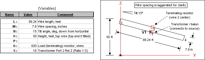
With the variables configured as shown and a 1 amp source, here is the current on Wire 2 (the wire with the 820 ohm terminating resistor in the center) at three different frequencies. (Exact results shown in the following illustrations may vary depending on which NEC engine is used.)
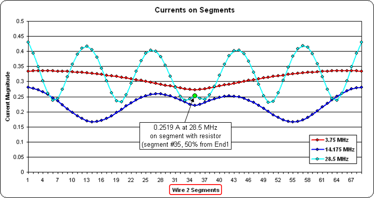
At 28.5 MHz the magnitude of the current through the terminating resistor is 0.2519 amps (green dot marker). For the other two frequencies shown the magnitude is similar at the center although it differs significantly at other points along the wire.
Now suppose you wanted to know the power dissipated in the resistor. Since the resistor is modeled as a load, one way to do that would be via the EZNEC "Load Data" window.
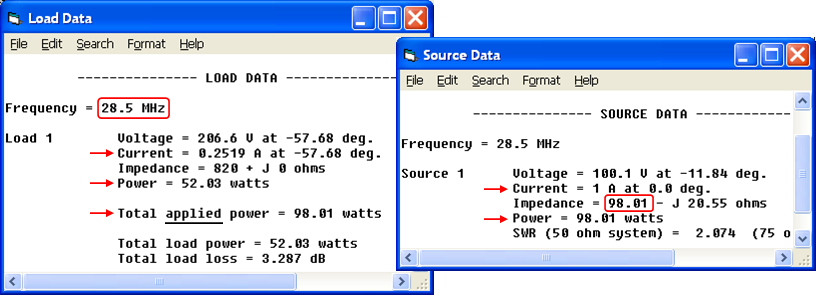
Note that 52.03 watts is the power lost in the load when the total applied (source) power is 98.01 watts. Where did the 98.01 come from? The model specified 1 amp current at the source. So:
Power = I^2 * RThe power at the source is therefore equal to the resistance at the source when the current at the source is 1 amp. But the source resistance, and hence the applied power, will change for each frequency as is shown by this portion of the AutoEZ Calculate sheet.
hence
SrcPower = SrcAmps^2 * SrcR
and SrcAmps = 1, so
SrcPower = 1^2 * SrcR
or just
SrcPower = SrcR
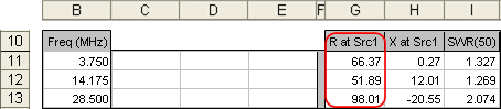
For example at 3.75 MHz the source resistance is 66.37 ohms. Hence the applied power is 66.37 watts with a 1 amp source. At 14.175 MHz the applied power is 51.89 watts with a 1 amp source.
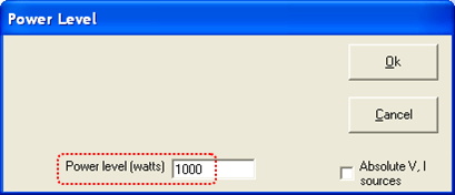
To even out the applied power at all frequencies, say at a level of 1000 watts, you can use EZNEC Options > Power Level. Uncheck the "Absolute V, I sources" option and set the desired power level.
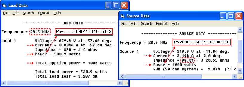
Now instead of 1 amp at the source, EZNEC will automatically recalculate the current (and voltage) at both the source and the load to be equivalent to 1000 watts of applied power. The recalculation is done "on the fly"; information in the "Load Data" and "Source Data" windows will change while the windows remain open.
As shown below on the right, at 28.5 MHz the source current will be 3.194 amps (not the original 1 amp). As shown below on the left, the load current will be 0.8046 amps (not the original 0.2519 amps) and the load power will be 530.9 watts (not the original 52.03 watts). However, note that the power at both the source and the load is still
I^2 * R .
Caution: If you set an explicit input power level, that setting will remain in effect until you close EZNEC. So if you open a different model with a 1 amp current source you may wonder why all the reported currents are not as you expected. For the remainder of this example it is assumed that you've set the EZNEC Power Level back to "Absolute V, I sources".
To find the power lost in the load for a given input (applied) power, an alternative to using the EZNEC "Load Data" and "Power Level" windows is to calculate the data directly in AutoEZ, taking advantage of custom function CurMag() along with the use of User-Defined Result Columns.
Custom function CurMag()
CurMag(WireNum, PctFromE1, TestCase)returns the current magnitude on a specified wire at a specified percent from end 1 for a specified test case. So in this example if we want the current in the load at 28.5 MHz, and the load is placed onWire 2 at 50% fromEnd 1 , and 28.5 MHz is test case 3 (row 13 on the Calculate sheet), then=CurMag(2, 50, 3) ===> 0.2519 amps (load current with 1 amp input)would return 0.2519 amps (assuming a 1 amp source). The load power isLoadAmps^2 * LoadR , and you know the LoadR to be 820 ohms, so the load power is=CurMag(2, 50, 3)^2 * 820 ===> 52.03 watts (load power with 1 amp input)noting that you can "square" a function call just like squaring a variable name.If you want to know the load power at a constant input power level, say 1000 watts, you can simply multiply that result by a factor of
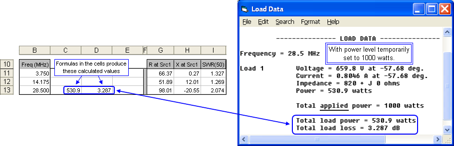
(NewAppliedPower / OldAppliedPower) or(1000 / SrcR) since, as explained above, the applied power with a 1 amp source is equal to SrcR. If the SrcR is found in cell G13, for example, the load power at 1000 watts input would be=CurMag(2, 50, 3)^2 * 820 * (1000 / G13) ===> 530.9 watts (load power with 1000 watts input and SrcR in cell G13)Furthermore, you can use that result to calculate the load loss in dB.Load loss dB = -10 * LOG10(1 - (LoadPower / InputPower))If the calculated load power is in cell C13, the load loss in dB can be calculated as= -10 * LOG10(1 - (C13 / 1000)) ===> 3.287 dB (load loss)Placing the formulas for "load power with 1000 watts input" and "load loss" in cells C13 and D13 on the Calculate sheet results in the values shown below on the left. Note that these values match the "Total load power" and "Total load loss" shown in the EZNEC "Load Data" window when the applied power was (temporarily) changed to 1000 watts, below right.
In the example above the third argument of the CurMag() function, the test case number "3", was set explicitly. Note that test case "3" is row 13 on the calculate sheet. Test case 1 is row 11, test case 2 is row 12, and so on. So instead of using
=CurMag(2, 50, 3)you could use=CurMag(2, 50, ROW()-10)ROW() is a built-in Excel function that returns the current row number, so when "ROW()-10" is used in a formula anywhere in row 11 the result is "1", when used anywhere in row 12 the result is "2", and so on. Hence "ROW()-10" is the equivalent of "Test Case Number". (For another example of using the ROW() function see Exponential Frequency Steps.)Now why would you want to go to all the trouble of using the CurMag() function, possibly combined with "squaring" and references to other cells and use of the ROW() built-in function? Why not just look at the EZNEC "Load Data" window?
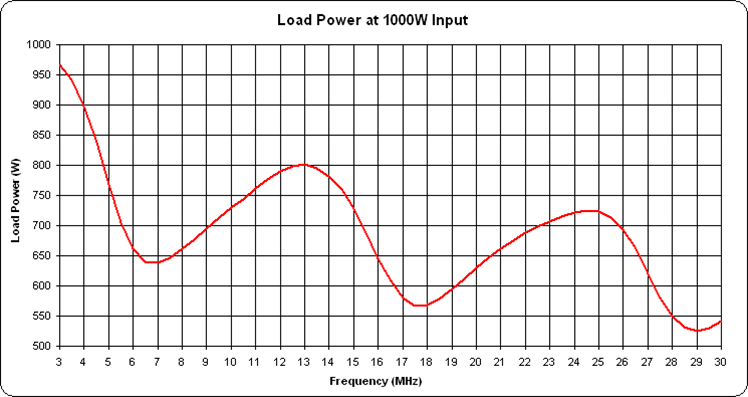
The advantage of doing the calculations in AutoEZ is that you can then set up a frequency sweep, easily duplicate the above cell formulas for all frequencies (all test case rows), and then plot the results. Here is the power in the load resistor at 1000 watts input over a frequency range of 3 to 30 MHz.
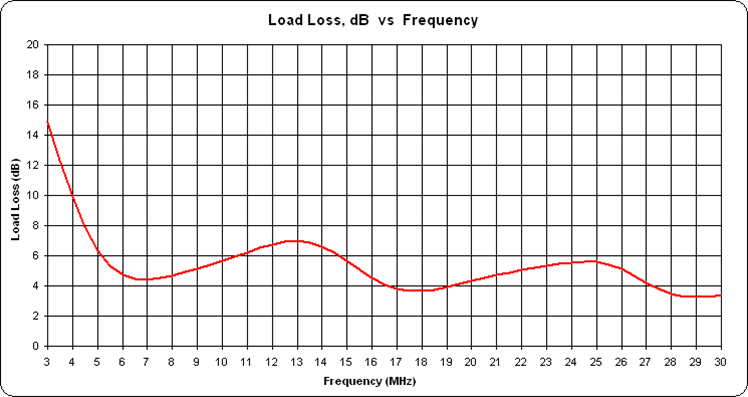
And here is the equivalent loss in dB.
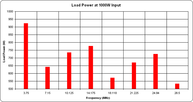
If you prefer you can do the calculations at discrete frequencies rather than over a range. For example, here is the load power on 8 bands.
When working with the CurMag() or CurPhase() functions, if you can't remember the argument list you can use the Excel "Insert Function" button. Click the "fx" just to the left of the formula bar, then select category "User Defined". (User Defined is another name for custom function.)
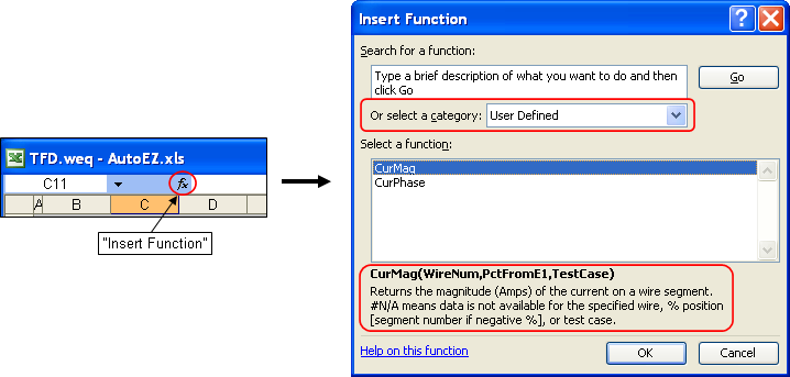
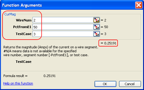
If you like you can then select one of the two functions and click OK. In the dialog that follows you can enter values for function arguments WireNum, PctFromE1, and TestCase. When you do so the function result (0.2519 amps in the illustration below) will appear. And if you click OK on that dialog the complete function call will be inserted into the currently selected cell.
Hint: If you want to specify an explicit segment number on a wire rather than a percent from end 1 value, use a leading minus sign
("-") followed by the segment number as the PctFromE1 argument.
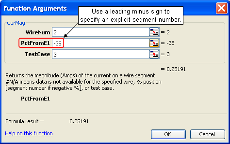
In this model wire 2 has 69 segments, so segment number 35 is the same as 50% from end 1.
Remember: Before running any calculations with AutoEZ make sure you have not set an explicit power level in EZNEC. Otherwise EZNEC will apply the power correction factor once and then AutoEZ will apply the same correction factor again.
Wire Insulation - Multiple Settings
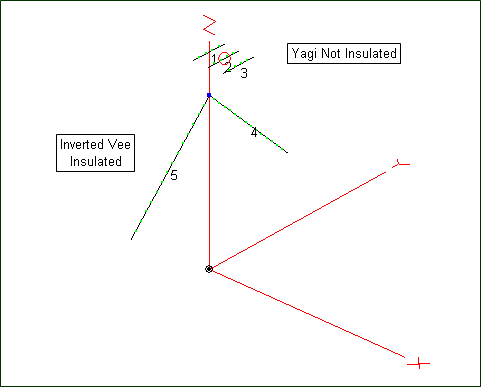
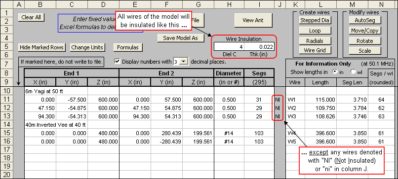
As of maintenance release v2.0.13 it is possible to have some wires of a model be insulated while other wires are not insulated.For example, suppose you have a model of a 6m band 3-element Yagi at a height of 50 ft (600 inches) combined with a 40m band inverted vee at 40 ft (480 inches). The Yagi is bare aluminum 0.5" tubing while the vee is #14 AWG copper with typical THHN insulation.
On the Wires sheet set the "Wire Insulation" fields (cells H5-I5) for the insulated wires of the model. Then indicate which wires are not insulated by entering "NI" (or lower case "ni") in column "J" for all wires which are Not Insulated.
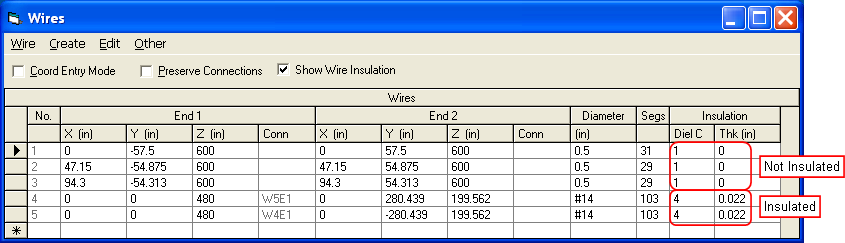
When the model is passed to EZNEC the insulation properties will look like this.
As of maintenance release v2.0.21 it is possible to specify multiple settings for those wires which are insulated. Follow these steps:
- Set the default "Wire Insulation" fields (cells H5-I5) to something other than 1 and 0.
- For any wires that should not use the default values, set the desired values in column "J". Use a semicolon to separate DielC and Thk. The semicolon must always be used even if one of the values is the same as the default.
- You can use numeric values or variable names for either DielC or Thk or both. Valid entries might be:
- 2.5;0.034 [DielC 2.5, Thk 0.034, both set as numeric constants]
- =B & ";" & D [both set via variables, B and D in this example]
- =G & ";" & 0.041 [DielC set with a variable, Thk set as a constant]
- If the column "J" cell for a wire is empty or does not include a semicolon that wire will use the default insulation settings.
As of maintenance release v2.0.30 you can also specify an (optional) insulation loss tangent value. Add a second semicolon followed by the loss tangent value. Note that when using the NEC-5 engine, EZNEC Pro+ v. 7.0.4 or later is required in order to recognize the loss tangent setting.
Note that the EZNEC restriction of supporting only a single wire loss value (copper, aluminum, etc) still applies. However, as stated in the EZNEC Help: "In the vast majority of typical antennas, wire loss doesn't cause enough difference to be of concern."
Smith Charts and SWR Charts for a G5RV / ZS6BKW
Both the G5RV and its newer cousin the ZS6BKW make use of a "matching section" of parallel conductor transmission line attached to the antenna feedpoint. A length of 50 ohm coax then completes the run to the station. In a discussion concerning the losses on that 50 ohm coax, W5DXP presented a depiction of a Smith chart with colored rings representing different SWR regions.
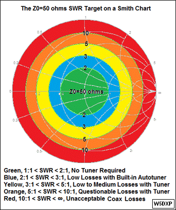
If the impedance at the junction of the matching section and the coax is plotted on a Smith chart, the idea is to show regions where the SWR(50) on the 50 ohm coax is acceptable or not acceptable.
Here are the modeled results looking into the matching section for a typical ZS6BKW antenna. This is a #12 diameter wire 92 ft long, at a height of 40 ft over average ground, fed with 40 ft of Wireman 551 ladder line (nominal Zo 400 ohms). To avoid clutter only the upper HF bands have been modeled. Annotations denote the high frequency end of each band. The green dot marker shows the impedance and SWR at 14 MHz.
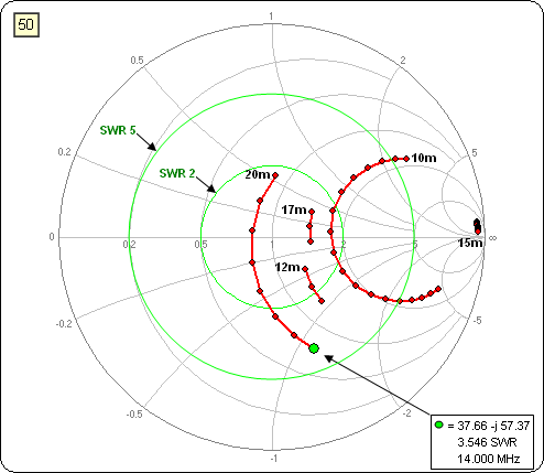
A Smith chart is really a plot of complex reflection coefficient values but with gridlines showing the corresponding complex impedance, typically normalized to 50 ohms. Note that "complex" means a quantity that has real and imaginary components. For impedance, the real component is resistance (R) and the imaginary component is reactance (jX).
The same idea of plotting one thing but having the chart gridlines show something else can be applied to the magnitude of the reflection coefficient, which is a scalar quantity rather than a complex quantity. Using a rectangular chart you can plot reflection coefficient magnitude (scalar) on the vertical axis but have the gridlines show SWR (also a scalar quantity).
In fact, an EZNEC "SWR chart" is actually a "reflection coefficient magnitude" chart but with "SWR" gridlines. Here is the EZNEC SWR chart using the same calculated frequencies shown on the above Smith chart. (The straight lines are just artifacts of frequencies not calculated. Ignore them.)
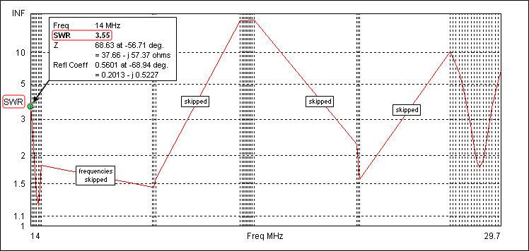
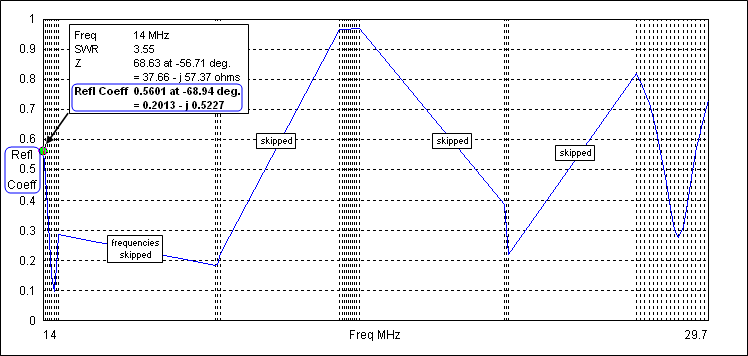
Some people mistakenly think that an EZNEC SWR chart has a logarithmic vertical scale. That's not true. The vertical scale is actually reflection coefficient magnitude but the gridlines are in SWR units. If you have EZNEC+ or EZNEC Pro (not Standard or Demo) you can plot the same data but with reflection coefficient gridlines. Notice that the shape of the plot is exactly the same; only the gridlines have changed.
AutoEZ can show the same kind of rectangular chart except that AutoEZ shows both gridlines types; reflection coefficient on the left and SWR on the right. Here's AutoEZ's version. Again, annotations denote the high frequency end of each band. And just to come full circle, the W5DXP colored SWR regions are included.
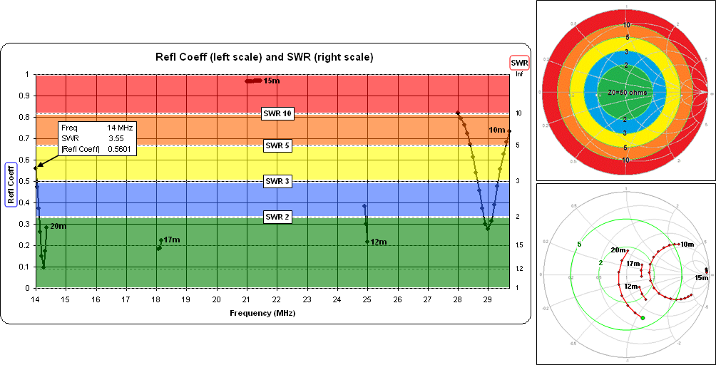
Perhaps this helps clarify the relationship between Smith charts and SWR charts.
Here's the model used for this exercise.
For an explanation of why the impedance gridlines on a Smith chart are shaped like circles and arcs see:
Speedometers, Thermometers, SWR Meters, and Smith Charts
Combined Ladder Line plus Coax Loss for a G5RV / ZS6BKW
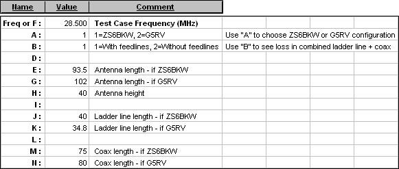
Related to the previous example, here are the SWR values at the station end of the feedline (combined ladder line plus coax) for both a ZS6BKW and a G5RV on 8 bands. That is, this is the SWR that a tuner would have to handle. (The ZS6BKW model for this example has a slightly different wire length compared to the previous example.)
The model used in this example has a single variable "A" which can be used to easily switch between the ZS6BKW and G5RV configurations. A second variable "B" makes it easy to switch the source position between the input end of the combined feedline (used to produce the illustration above) and the antenna feedpoint (thus removing the feedlines from the model). Here's a portion of the AutoEZ Variables sheet tab.
To calculate total feedline loss first run the model with feedlines included (B=1). On the Calculate sheet, copy the computed gain values (cells J11-J18) down to empty lower rows. Change the model to without feedlines (B=2) and run it again. For any given frequency, the delta between the current computed gain value (without feedlines, B=2) and the previously copied gain value (with feedlines, B=1) is the feedline loss. That delta is plotted below. (Also see the next example for more on how to compute the feedline loss.)
Here's the "switchable ZS6BKW/G5RV" with "removable feedlines" model.
A very complete analysis of the differences between the ZS6BKW and the G5RV was done by K4SAV in this thread on qrz.com. The above example was a small part of that thread. Also see the G5RV pages by G3TXQ and W8JI.
General Purpose Flat/Vee/Catenary Doublet with Ladder Line Feed
Another very popular multiband antenna is a doublet fed entirely with ladder line all the way back to the shack, or perhaps to a tuner just outside the shack window. This is an analysis of such a system.For this example a general purpose model having the following set of variables was used.
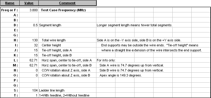
With this model you enter the center height, the heights at the tie-offs (which may be beyond the wire ends), and the horizontal span between center and tie-offs. Excel formulas then use the necessary sine and cosine functions to translate your entries into the appropriate X/Y/Z wire coordinates.
If you set the center height higher than the tie-off heights the model will be an inverted vee. If you set all three heights equal the model will be a flat dipole. If you set the center height slightly lower than the tie-off heights the model will have a "catenary sag" in the middle.
You are free to make the model asymmetric if desired by using two different values for the side A and side B tie-off heights. So you could make an inverted vee with the two legs having different angles. Or you could make a sloping dipole by having one tie-off higher than the center and the other tie-off lower.
Looking down on the antenna from above, if the wire is not in a straight line you can use variables "N" and "O" to make a dog-leg shape or a vee shape.
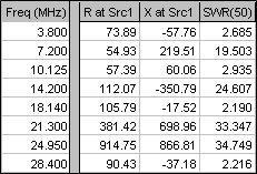
With the model configured as shown above here are the impedance values as seen at the input end of 104 ft of Wireman 552 ladder line (Zo ~380 ohms, VF ~0.917). In other words, these are the impedances that the tuner has to convert to 50+j0 ohms.
I chose that particular set of frequencies to be the same as those used by the W5DXP IMAXGRAF tool. Here's what that tool shows, with a line length of 104 ft marked in red.
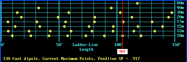
With IMAXGRAF the yellow dots indicate "easy to match" impedances with an SWR(50) less than 3:1. Half-way between dots are "harder to match" impedances. Pretty good correlation given the fact that IMAXGRAF assumes a flat dipole and 450 ohm ladder line.
Here is the dB loss in the 104 ft of ladder line for each band.
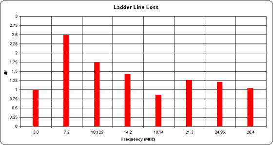
To compute these loss figures I first copied the calculated "Max Gain" values down to lower rows on the Calculate sheet, being sure to leave a few extra blank rows. Then I temporarily removed the transmission line from the model, changed the source placement to Wire 2 / 50% (the antenna feedpoint), and re-ran the calculations. (The model can be reconfigured with/without the transmission line via use of variable "T".)
After this second set of calculations I entered a set of formulas to find the difference in the "before and after" Max Gain values for each frequency. If nothing has changed in the model except for the removal of the transmission line then the difference in gain equals the loss in the line. Here's a marked-up Calculate sheet to illustrate. Gain values are for an elevation slice at 0° azimuth. It doesn't matter what plot type or angle is used as long as the choice is not changed between "before" and "after". Note that I also changed the SWR reference Z from 50 to 380 ohms to show the appropriate SWR at the antenna feedpoint.
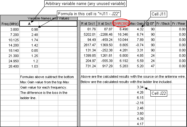
For more information on the use of output or results variables such as "A" above see section "User-Defined Result Columns" here.
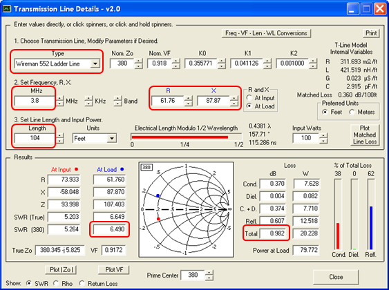
The ladder line loss values are (almost) exactly what you would see using TLDetails; at 3.8 MHz, 0.98 dB above as calculated by EZNEC, 0.982 dB below as calculated by TLDetails.
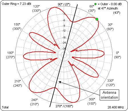
So much for impedances at the tuner and losses in the transmission line. The next part of the analysis is to study the radiation patterns. For reasons that will become clear in a moment I first used the "Rotate" button on the Wires sheet to rotate the entire antenna 15° clockwise looking down from above. The wire is still straight (from the top down view) but the physical alignment is now from 15° east of north to 15° west of south, representing the actual orientation of the antenna in this study. With that done, here's the azimuth pattern for 28.4 MHz at an arbitrary TOA of 20°. The azimuth angle numbers in parenthesis are compass (actually true north, not magnetic) values, added by using the "Secondary Azimuth Labels" button on the Patterns sheet tab.
And here's an animation of the azimuth patterns at an arbitrary TOA of 20° for all the bands. Frequency is shown in the lower right corner. The outer ring is frozen to allow comparison of relative pattern strength as well as shape.
Now why would I want to go to the trouble of reorienting the antenna like that? Well, NS6T has a very nice web page that can produce azimuthal projection maps centered on any arbitrary location. I created one using the lat/lon of a Texas location (again representing the antenna used in this study) then used that map as the background image for the polar plot.
On 10m this particular antenna should have a nice signal into Western Europe, not so great to the Australian coastal population centers.
The final part of the analysis is a study of the antenna efficiency. AutoEZ can calculate Efficiency / Loss / Average Gain Test automatically, unlike in straight EZNEC where you have to manually remove all loss factors from the model.
Here are the efficiency numbers for a 102 ft G5RV compared to this 130 ft doublet. The loss factors taken into account are a) ground loss, b) antenna wire copper loss, and c) transmission line loss. For the G5RV the transmission line consisted of ~130 ft of RG-8X and 31.3 ft of window line "matching section". Not included in either case are any balun losses and tuner losses.
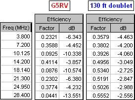
And here's a corresponding graphic comparison. Since this is efficiency, not loss, higher is better.
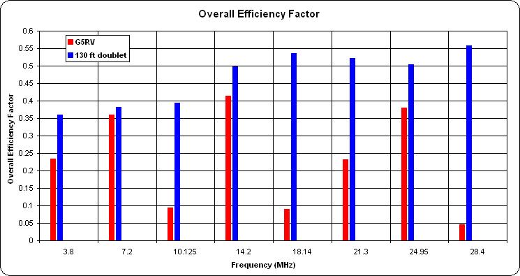
On several bands the difference is dramatic.
Here's the flat/vee/catenary model used for this study.
For an explanation of the math behind the efficiency values see the last section on this page.