View a Single 3D Plot
AutoEZ offers several ways for you to work with 3D data for your model. On the Calculate sheet the 3D Plot (For Selected Row) button will build a model using the frequency and variable values (if any) for the row containing the Excel selection cursor, then send that model to EZNEC with instructions to run the NEC engine and display a 3D plot. You may place the Excel cursor in any column on either the left or right side of the sheet. It is not necessary to calculate the row beforehand.
After you have calculated one or more rows the Patterns sheet will be visible. On that sheet the 3D Plot for this Test Case button will produce an EZNEC 3D plot for the test case (row) that is currently being shown. You can use the spinner to cycle through all available test cases or you can type a number directly into the "Test Case" cell.
Sometimes it is helpful to see both the wires of the model and the 3D radiation plot at the same time. EZNEC has a powerful feature for this situation and AutoEZ makes it easy to invoke that feature. On the Calculate sheet the Both in Sync (For Selected Row) button does just what the name implies. Using the frequency and variable values (if any) for the selected row, AutoEZ will build a model and send it to EZNEC with instructions to first run the NEC engine, then show the View Antenna window, then also show the 3D Plot window. AutoEZ then manipulates the size and position of these two sub-windows such that they are side-by-side and span almost the entire desktop.
By default, AutoEZ will instruct EZNEC to highlight an elevation slice on the 3D Plot window. You can change the highlight to an azimuth slice or set highlighting off. The same slice that is highlighted in red on the 3D Plot window will show as black on the View Antenna window (if using the default EZNEC colors). As you use the slider on the 3D Plot window to change which azimuth or elevation slice is highlighted, the slice shown on the View Antenna window will track your selection.
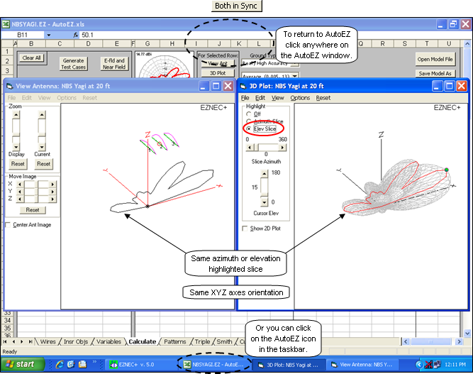
You can drag with the left mouse button on either window to change the orientation of the image. You can also use the keyboard arrow keys. When you release the mouse button (or arrow key) the "other" image will snap to the same axes orientation. The animation below illustrates this. One graphic (either one) is being rotated about the Z axis. When the mouse button or arrow key is released the other graphic follows.
(Press Esc to stop the animation, F5 to restart.)To return to AutoEZ there is no need to explicitly close the two EZNEC windows. Just click anywhere on the AutoEZ window, visible in the background, or click on the AutoEZ icon in the taskbar.
View Multiple 2D Slices
When viewing an EZNEC 3D plot, if you highlight an azimuth or elevation slice you can also show the EZNEC 2D plot for that slice. For example, this shows the azimuth slice at 15° elevation highlighted on the 3D plot and the corresponding 2D azimuth plot at that elevation angle.
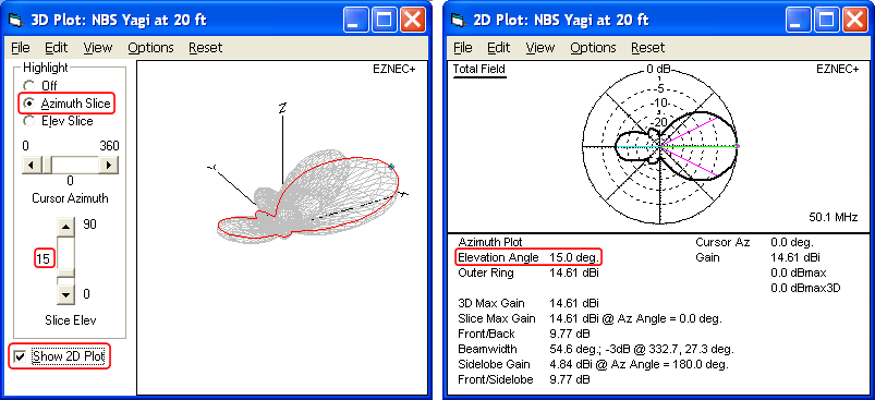
Using the "Slice Elev" scroll bar you can select a different slice to highlight; however, you will be limited to the step size used for the 3D plot, 5 degrees in this case.
An alternative way to show different 2D slices is to use a variable to control the plot angle on the AutoEZ Calculate sheet. Variable AA is shown below but any unused variable name will do. Then on the Patterns sheet you can step through the test cases to see the pattern at different angles. (This feature added as of AutoEZ update 2.0.12.)
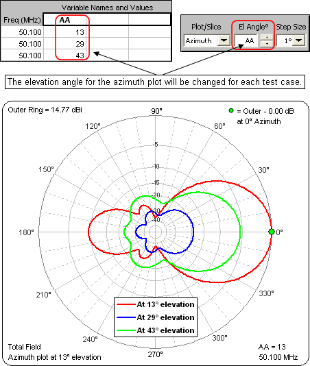
Above, the elevation angles corresponding to the first pattern peak (at 13° elevation), the first pattern null (at 29° elevation), and the second pattern peak (at 43° elevation) are shown.
Calculate 3D Data
When you select the Include 3D Data in Calculations option on the Calculate sheet AutoEZ will instruct EZNEC to build an OpenPF format (.PF3) file for each calculated row in addition to doing the normal calculations. AutoEZ will then read that PF3 file to determine the 3D Max Gain and the Az/El angles for that max gain point, along with the Average Gain and the Receiving Directivity Factor (the difference between the 3D Max Gain and the Average Gain).
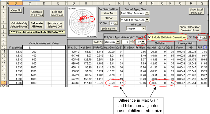
The example above is for a 160 meter Beverage antenna for seasonal use in the winter months, suspended on bamboo stakes 6 feet above a farmer's field. The main wire is being varied in length (using variable L) from 200 feet to 1800 feet. Note that the max gain and the angle of that max may vary slightly between the "Slice" columns
(J-K) and the "3D" columns(N-O-P) , depending on whether you have chosen the same or a different step size for each.If you wish you can verify the AutoEZ 3D data directly in EZNEC. Select any cell in the desired row and click the AutoEZ 3D Plot (For Selected Row) button. In this case, when you wish to verify the 3D data, make sure the step size used for plotting matches the step size used for data. In the general case it is not necessary to have these two step sizes be equal.
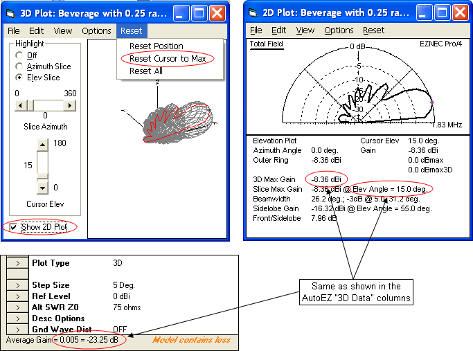
In the EZNEC 3D Plot window highlight a slice (elevation in this case) and then click Reset > Reset Cursor to Max if necessary. Then click the "Show 2D Plot" option box. In the EZNEC 2D Plot window click View > Show Data if necessary. The data shown on the 2D plot along with the Average Gain shown at the bottom of the EZNEC main window will be the same as is shown by AutoEZ.
As of maintenance release v2.0.22, if the 3D step size is 1° and the ground type is other than Free Space a "type 13" IONCAP/VOACAP file will be created automatically for each test case row. The files are named
"$AEZ$nnn.13" where "nnn" is the test case number. For example, if you calculate three test case rows files"$AEZ$001.13", "$AEZ$002.13", and"$AEZ$003.13" will be written to the AutoEZ home folder, typicallyC:\AutoEZ. You can rename these files and/or move them to other folders as desired. Any such"$AEZ$nnn.13" files that are present in the home folder will be deleted when a new model file is opened or when the calculation results are cleared.The azimuth patterns in the type 13 files will be automatically rotated if necessary such that the angle of maximum gain points to the "North" (0°) compass direction. This is equivalent to the EZNEC "Pattern Maximium" option.
View a Sequence of 3D Plots
After you have included 3D data in the calculations a new AutoEZ button will appear, Show 3D Plots for Calculated Rows. This button makes use of the EZNEC TraceView mode to view (in 3D format) the contents of the OpenPF PF3 files that were generated as part of the AutoEZ calculations.
When you click the button AutoEZ will a) put EZNEC into TraceView mode and minimize the EZNEC window, b) create a small "postage stamp" dialog window in the lower-right corner of your desktop, c) instruct EZNEC to show a TraceView 3D plot for the first available PF3 file. You can then use the spin button on the "Select 3D Plot" postage stamp dialog to cycle through all the PF3 files. You can resize the 3D plot window and change the axes orientation as desired. The axes orientation will "persist" from one plot to the next.
The animated GIF shown below illustrates what it means to view a sequence of 3D plots. In actual operation EZNEC must close and then redraw the 3D plot window for each new plot.
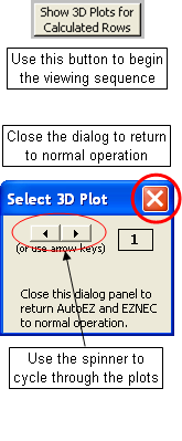
(Press Esc to stop the animation, F5 to restart.)To return both AutoEZ and EZNEC to normal operation just close the "postage stamp" dialog window.
There may be times when you want to use a smaller 3D step size of 1° or 2° in order to get more resolution in the calculated results shown in columns N through S. You can use this small-step data with the Show 3D Plots button and EZNEC TraceView but the 3D plots will be less than optimal. To accommodate this situation, when the PF3 file has a step size of 1° or 2° you will see a Sparse Gridlines checkbox. If you select this option AutoEZ will create a temporary PF3 file just for viewing which has a 6° step size. (If the original PF3 file has a step size of 5° or 10° the Sparse Gridlines checkbox is not shown.)
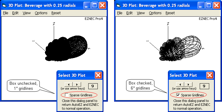
Dense (1°) gridlines on the left, sparse (6°) gridlines on the right.
The "View a Sequence of 3D Plots" feature is not available when using Excel 97.
Calculate Efficiency / Loss / Average Gain Test
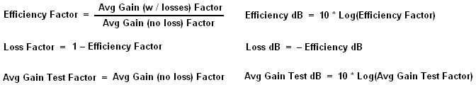
When you select the optional With E/L/AGT checkbox AutoEZ will, in addition to doing the normal 3D calculations, build a temporary model file with all loss elements removed. That is, the model will have no ground loss, no wire loss, no load loss, no transmission line loss, and no L network loss. This model is sent to EZNEC with instructions to create a "no loss" PF3 file. AutoEZ reads this file then calculates and stores the "no loss" average gain, which is also called the Average Gain Test value. This value can be used with the previously-calculated average gain "with losses" value (column Q) to calculate overall system efficiency and overall system loss, and is used directly to show the Average Gain Test value, via the following relationships:
Use the small E/L/AGT button to cycle through showing Efficiency to Loss to Average Gain Test values. To assist you in keeping track of what is shown the color of the column headers will change as well as the text, with Efficiency in black, Loss in red, and Avg Gain Test in blue. You can cycle at will through the three different meanings for columns T-U. It is not necessary to recalculate the row or rows.
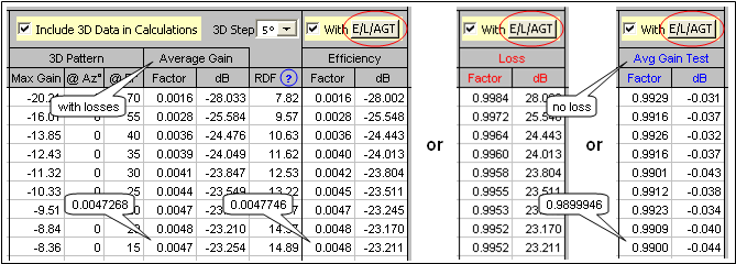
In the example above you may think that the values have been calculated incorrectly but keep in mind that this is a Beverage antenna with very low efficiency (very high loss). More precise values are shown in the balloons which you can use to verify the calculations.
For additional information look in the EZNEC Help. On the Index tab, enter keywords "efficiency" or "average gain".
LB Cebik, W4RNL, has created some guidelines for Average Gain Test values. In terms of the absolute value of the AGT dB level, Cebik's guidelines are:
- |AGT| < 0.2 dB: "Model is considered to have passed the test and is likely to be highly accurate."
- |AGT| > 0.2 dB: "Model is quite usable for most purposes."
- |AGT| > 0.4 dB: "Model may be useful, but adequacy can be improved."
- |AGT| > 0.8 dB: "Model is subject to question and should be refined."