
This AutoEZ examples page is devoted entirely to modeling SteppIR Yagi antennas. Additional sections may be added in the future as the need arises to discuss more advanced topics.
If you are not familiar with AutoEZ please take a moment to look over the Quick Start Guide. Otherwise, the information on this page probably won't make much sense.
SteppIR Yagis - Basic Setup
Models have been developed for each of the SteppIR Yagi antennas:
See the zip file at the end of this section to download the model files.
- 2E
- 3E
- 4E
- DB11
- DB18
- DB18E
- DB36
- DB42
- UrbanBeam
- DB32 (discontinued, not shown below)
- MonstIR (original straight element design, discontinued, not shown below)
To help identify what's what here is an extract from one of the SteppIR brochures.
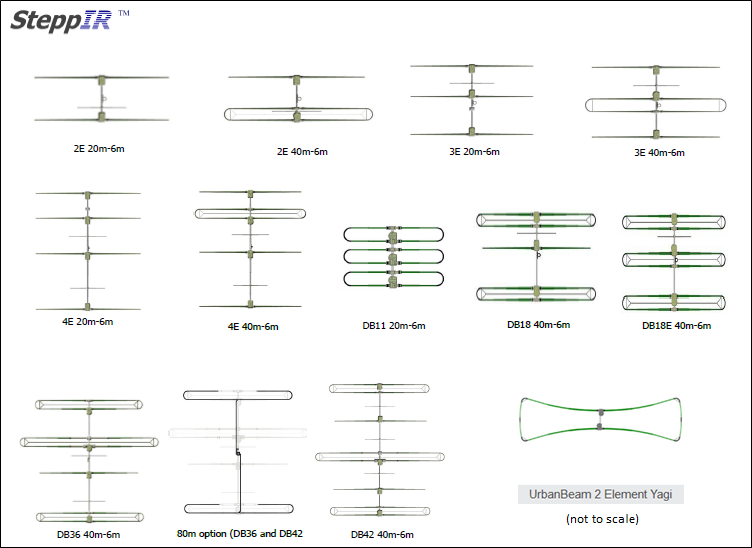
For each antenna, a single AutoEZ model covers all bands and all options that are available for that particular Yagi (optional 40/30m dipole loop with the 2E, 3E, and 4E; optional 80m dipole with the DB36 and DB42; optional 6m extra passive elements with all except the DB11 and UrbanBeam).
With any given Yagi the wires of the AutoEZ model are automatically reconfigured as the frequency is changed. In addition, the feedpoint is automatically changed if necessary for different bands and/or as the model is switched from Normal (Forward) to 180 (Reverse) to Bidirectional mode. Below left is an animation of how the wires of the DB42 model change from 40m to 6m. Notice the feedpoint switch at 14.175 MHz. Below right shows how the wires of the UrbanBeam change over the same frequency range.
Just for fun, this link shows an UrbanBeam doing a pretty good imitation of a dog chasing its tail. As the driven element tape (left, with red circle) spools in the director tape (right) spools out giving chase. And vice-versa.
After using the Open Model File button to load a particular model the first thing you should do is change various default settings to match your scenario.
1) On the Wires tab: With one exception to be discussed later, no changes need be made on the Wires tab. All the XYZ coordinates and other details for all the wires are set automatically as a result of changes to variable values.
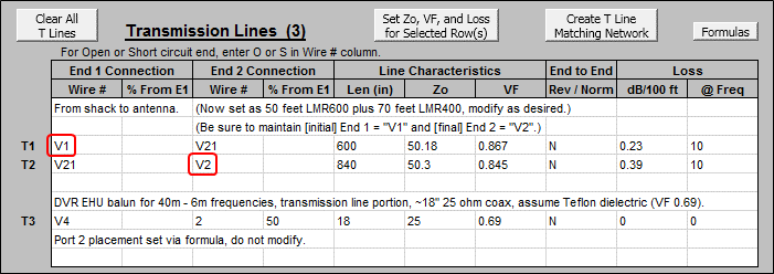
2) On the Insr Objs tab: Change the transmission line type(s) if desired. You can use a single line type for the entire run from shack to antenna or you can break that run into multiple line types. However, be careful to always maintain the "shack end" as V1 and the "antenna end" as V2. The default entries look like this.
To use just a single length of, for example, 100 feet of RG-213 the entries would look like this.
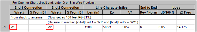
To set the line characteristics you can first select any cell in the appropriate row and then click the Set Zo, VF, and Loss for Selected Row(s) button. You will be able to choose from approximately 100 different line types. Don't forget, the line length(s) must be set in inches not feet. You can enter an Excel formula in the "Len" cell if you wish, for example
"=100 * 12". Do not modify the final entry shown in the table.If you do not want to include any shack-to-antenna transmission lines just delete both the first two entries and then change the source from V1 to V2. Or, if you only want to temporarily remove the transmission lines you can "mark them out" by placing an "x" or any other non-blank character in column A of the associated table row, along with changing the source position. To put the transmission lines back into the model just clear the marks and set the source position back to V1. (With Excel, a cell is cleared by first selecting it and then pressing the keyboard Delete key.) Again, do not modify the final entry shown in the table.
3) On the Variables tab: Change the Height. The appropriate variable name differs with different models. Look for the column D comment "Height above ground (now 65 ft)". As you reset the Height in inches the comment will change to reflect the height in feet. Also note that all dimensions for all models are in inches. Currently there are no corresponding metric models; units must remain as inches.
Still on the Variables tab, follow the instructions in cell F13 to set certain variable values to zero if you do not have the optional 6m passive element(s) kit. On the other hand, if you do have the optional 80m dipole for the DB36 and DB42, change certain variable values from zero to the values shown in the comments.
Finally, look over the notes starting in cell F20. The tape length table entries match the factory default settings for the Mustang controller firmware level. If you are not using that firmware level, or if you have made custom changes to any tape lengths, you can modify the corresponding table entries to match. Below is a portion of the Variables tab for the DB18E model.
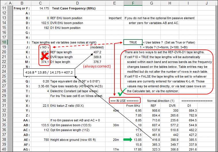
As you are working with a model make sure you keep track of the value in cell F18. If F18 is TRUE then the values shown for variables K, L, and M are ignored. The tape lengths used to construct the model will be as interpolated from the appropriate table entry. For example, in the screen grab above the current frequency (cell C11) is 14.175 MHz. So for the REF tape length, first the table entry for the 13.85 MHz band segment is found (416.8 inches) and then that value is scaled to the correct frequency
(416.8 * 13.85 / 14.175). This action corresponds to the Autotrack mode of theSDA 100 controller with the step size setup option set to 1 kHz.If you set F18 to FALSE, the table entries are ignored and the model will be configured per the values as currently set for K, L, and M. Set
F18 = FALSE if you want to experiment with adjusting the element lengths or if you want the lengths to stay fixed when you run a frequency sweep.
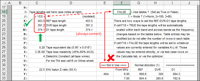
Whichever method is used to set the tape lengths, the values shown under "(modeled)" will always match the current model configuration.
Note: The REF/DVR/D1 element names are what would be shown on the
SDA 100 controller. For many of the SteppIR Yagis the actual "driven element" may change depending on the frequency and mode. For example, with the DB18E on 40m, in Normal and Bidirectional modes element D1 is the driven element. In 180 mode element REF is the driven element. On all other bands in all modes element DVR is the driven element.If you click the View Ant button to show the wires of the model you can see which element is being driven at the current frequency (cell C11) and mode (cell F19). If the driven element is not obvious, on the EZNEC View Antenna window click View > Objects then enable the "2 Port Objects" option. And here's a tip for EZNEC v6 users. On the View Antenna window, press keyboard key "z" to get a top-down view of the wires. Then press "c" to center the wires in the window.
4) On the Calculate tab: Change the dropdown selections for Ground Type and Ground Characteristics as desired then click the Calculate All Rows button. When the calculations are done switch to the Patterns tab and use the spin button to "watch the movie" of the changing azimuth or elevation patterns.
For example, the animation below shows the Free Space azimuth patterns (at 0° elevation) for the DB18E from 40m to 6m. The frequency for each frame is shown in the lower-right corner. The shack-to-antenna transmission line has been temporarily "marked out".
Here is a portion of the Calculate tab showing the details for each of the 8 patterns.
If you are satisfied with your changes you can then save the model, perhaps using a different name such as "My DB18E.weq" or "DB18E Free Space.weq" or some such other descriptive name.
Models:
SteppIR_Yagis.zip Note that units must remain as inches.
Unzip and save to your computer then use the Open Model File button from within AutoEZ.
Correlating to Measured SWR
When modeling SteppIR Yagi antennas the largest unknown is the effect of the CPVC guide tubes and fiberglass support tubes. Both act as a type of "wire insulation" surrounding the copper tape. The properties of that "effective insulation" will change the relationship between the physical length of exposed tape as set by the controller and the electrical length of the tape which determines the antenna response. The properties of the "effective insulation" vary somewhat with frequency and I am unaware of any way to empirically calculate what the properties should be.The AutoEZ models address this concern by implementing a frequency-dependent lookup table of "effective insulation thickness" values while keeping the insulation dielectric constant fixed at a default value of 4. The lookup table is found on the Wires tab following all the XYZ coordinate entries. For example, the table for the DB18E model looks like this.
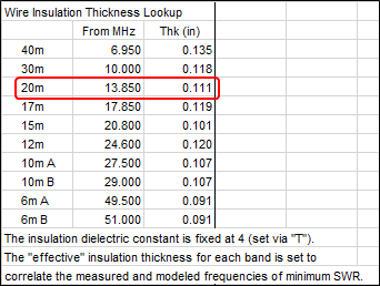
As the modeled frequency changes, the corresponding "band" entry will be used for the wire insulation thickness. Unlike with the tape length tables on the Variables tab, no scaling of the thickness is done within a band. The changes are strictly band-by-band and the values will typically be close to 0.1 inches. For the DB18E on 20m the default thickness is 0.111 inches.
If desired you can modify the table entries by measuring the SWR over a particular band using a VNA or antenna analyzer type instrument, noting the frequency of minimum SWR (the "dip" in the curve), and then changing the "effective insulation thickness" value in the table such that the frequency of the modeled dip matches that of the measured dip. Changing the effective insulation thickness is roughly analogous to setting a "Band Correction Factor" with the
SDA 100 controller. With the controller you are changing the physical tape lengths. With the AutoEZ model you are keeping the tape lengths the same but changing a different parameter that affects the electrical performance. With both the result is to "move" the frequency of the SWR dip.Still using the DB18E as an example, here is what the modeled SWR curves look like at three different values for effective insulation thickness. All three modeled sweeps were done with the tape lengths fixed at the 14.175 MHz scaled lengths. That is, on the Variables tab with F18=TRUE set the frequency to 14.175. Note the "(modeled)" lengths and manually enter those exact lengths for variables K, L, and M. Then set F18=FALSE so the lengths will not change when you run a frequency sweep on the Calculate tab.
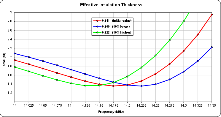
For this model and on this band, changing the effective insulation thickness by ±10% changes the frequency of minimum SWR by about ±50kHz. A thinner amount of insulation increases the dip frequency and a thicker amount decreases the dip frequency.
Now suppose you measured the SWR on 20m and found the "dip" frequency to be 14.1 MHz, or perhaps 14.3 MHz, or maybe even out of band at 14.4 MHz. How could you use that information to fine-tune the AutoEZ model?
The first step is to make absolutely certain that the tape lengths set by the controller match those set by the AutoEZ model at any given frequency. You can do that by putting the controller in manual mode, setting the frequency to the start of the segment for the 20m band (13.85 MHz), and then using Create/Modify for each of the three elements to display the controller's version of the tape lengths. If those lengths don't match the AutoEZ table you can either change the controller or change the tape length table entries for the 13.85 MHz row (on the Variables tab) in the model. If you change the controller you will of course have to measure the SWR again.
After that, freeze the modeled tape lengths (explicitly set K, L, M and set F18=FALSE) at whatever they were when you did the SWR measurement. In the example above that would be tape lengths that correspond to 14.175 MHz. Then do frequency sweeps similar to above while experimenting with different values for the effective insulation thickness. Make the sweep range a few hundred kHz on either side of the measured dip frequency so that you can see when the modeled dip starts to get close. To help keep track of the different insulation thickness values that you try you can use the Snapshots button on the Custom chart tab. And to accentuate the dip you can use the Set/Lock Scales button to "zoom in" the vertical scale.
For example, let's say the measured dip was at 14.3 MHz. Run sweeps from 14.100 to 14.500 MHz and use a fairly small step size, say 0.010 MHz. Before running each sweep set the insulation thickness to a different value; after running the sweep use the Snapshot button to capture the trace for that particular thickness. With just a few iterations you will be able to "home in" on what the insulation thickness should be for that band in order to make the modeled response closely match the measured data. The modeled chart might look something like this, with the vertical (SWR) scale set from 1.6 to 1.3 in order to make the dip appear sharper.
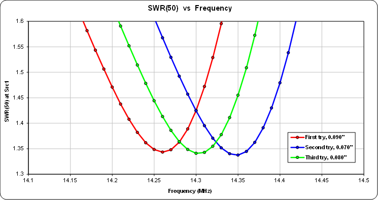
The first try was with an insulation thickness of 0.090 inches. That didn't move the dip frequency quite enough. The second try was with a thickness of 0.070 inches. That went a little too far. The third try was at 0.080 inches and that makes the model exactly match the measurement.
An Easier Way:
Now that you've seen the relationship between insulation thickness and frequency of minimum SWR, and seen how to adjust the thickness value in order to make the model coincide with actual measurements, you may be wondering if you have to go through the same steps of freezing the tape lengths and running iterative frequency sweeps in order to set the effective insulation thickness for other bands.
No, you don't. The AutoEZ optimizer can make short work of the process. Using the same example scenario as above, a DB18E on 20m with a default insulation thickness value of 0.111 inches for that band, here's how to use the optimizer to quickly determine the correct thickness value.
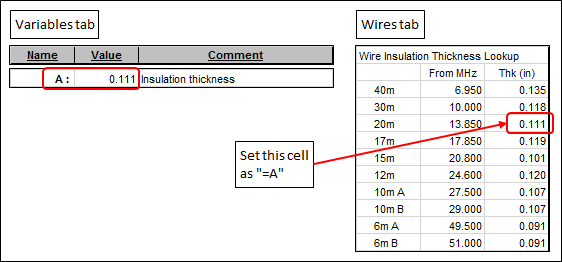
As before, start by verifying that the tape lengths as set by the controller are the same as those set by the model. Then pick an unused variable name on the Variables tab. Variable A is a good choice since A is not used by any of the AutoEZ models. Set the initial value for A as 0.111. Still on the Variables tab make sure F18=FALSE, tape lengths frozen at whatever they were when the SWR measurement was made.
On the Wires tab, set the insulation thickness for the 20m band using the Excel formula "=A". Hence as the value for A is changed, either by you manually or by the optimizer automatically, the corresponding entry in the lookup table will change.
Back on the Variables tab, click the Optimizer Setup button. Select variable A and make sure no other variables names are selected, then click OK. The Optimize tab will appear. On that tab, set the frequency to the measured frequency of minimum SWR, 14.3 MHz in this example. Set the target weight for SWR as 1 and clear all the other target weights (or set them all to zero). Make sure that the final values will be rounded to at least 3 decimal places.
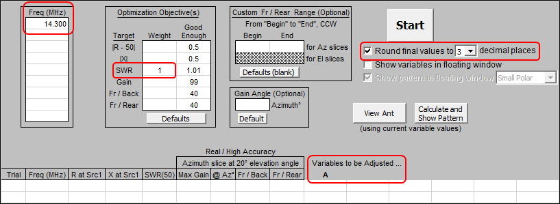
When you click the Start button here's what will happen. First, the frequency will be set to 14.3 MHz. But because F18=FALSE on the Variables tab, setting the frequency will not change the tape lengths. Then the optimizer will try different values for A, all at the same frequency, while seeing which values result in a lower SWR. When the optimizer can't find a setting for A that produces a lower SWR than some previously-tried setting it quits and sets A to whatever value produced the lowest SWR.
That's exactly what you want. The measured SWR was lowest at 14.3 MHz. The AutoEZ optimizer will work through different values for A until the modeled SWR is also at its lowest possible value at the same frequency. The whole process will take just a few seconds.
In graphical terms here is what the optimizer has done. Note that the horizontal axis is now insulation thickness, not frequency.
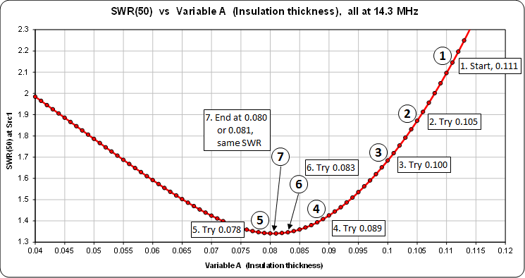
The steps labeled 2 through 7 represent those optimizer trials that resulted in a lower SWR value. Other trials (not shown) that resulted in a higher SWR than had been found already are discarded.
Be aware that the final value selected for A may vary in the last digit for different optimizer runs at the same frequency. That's because the optimizer rounds calculated SWR values to 3 decimal places. So if one value of insulation thickness produces a calculated SWR of 1.3408 and another thickness calculates out to SWR 1.3407, the optimizer will not waste time trying to distinguish between the two.
The only thing left for you to do is return to the Wires tab and type in the numeric value that is now shown for the 20m band, replacing the "=A" formula with explicit digits. If you have measured SWR curves for other bands you can put the "=A" formula in the new band position you wish to adjust, change the tape lengths on the Variables tab to match what they were for the SWR measurement on the new band, return to the Optimize tab and change the frequency to that of the measured SWR dip on the new band, and click Start again. When the optimizer finishes this time, again replace the "=A" formula on the Wires tab with the actual calculated digits. When you have no more bands to adjust clear (via the Delete keyboard key) A and its descriptive comment since that variable is no longer being used.
There is one caveat when using the optimizer to adjust the insulation thickness values. For very small thicknesses, typically found on 6m, while working through different values the optimizer may try a negative value. That will stop the process since the temporary model that would normally be sent to EZNEC for calculation is now invalid; it has a negative insulation thickness.
There are two ways to deal with this. You can be "proactive" and avoid the problem by using
"=MAX(A, 0.01)" as the formula rather than the simpler "=A". That way, regardless of what the optimizer might suggest as a possible thickness, the setting in the table will never go below 0.01. Or you can be "reactive" and wait to see if the problem will even occur. If it does, just select the final row in the optimizer log, click Reset to Selected Log Row, and then click Start again. This time the optimizer will be far less likely to "overshoot" when trying different values for A.Using the optimizer to set the insulation values will be far, far faster than doing manual changes combined with frequency sweeps, even if you have to deal with an "overshoot to negative" once in a while.
Modeling the EHU Balun
Accounting for the balun that is inside the driven element EHU of the SteppIR Yagis turned out to be a bit of a challenge. In an ideal world the balun could be modeled just by using an EZNEC "Transformer" insertion object with a 50:22.5 (input:load) impedance ratio. But if the goal is to have the model match the electrical performance of the physical antenna as closely as possible that's not good enough.I was fortunate to be given measurement data taken on an actual SteppIR balun. A 22 ohm resistor was measured from 6 to 54 MHz and then placed across the load side of the balun, where the brushes are located that contact the copper tape for each half of the element. Then the impedance at the input side of the balun was measured, at the SO-239 where the transmission line to the shack is connected. Measurements were done with a
SARK-110 antenna analyzer; the test leads of the instrument had been "calibrated out".On the load side, everything beyond the resistor is considered to be "antenna". On the input side, everything before the
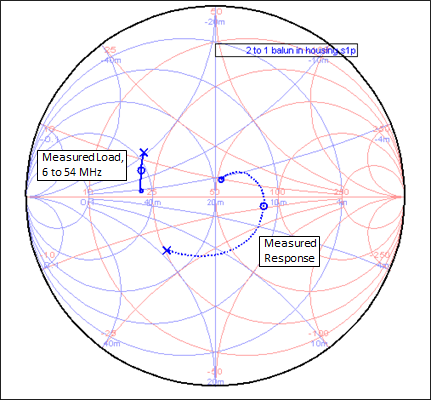
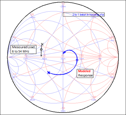
SO-239 is considered to be "transmission line to shack". Everything in between is called "balun" and that's what I wanted to simulate.The two measurement files were loaded into the SimSmith circuit simulator by AE6TY. Here is a Smith chart showing both measurements. The solid trace is the measured impedance of the load (the resistor). The dotted trace is the measured impedance at the SO-239, the input side of the balun. On both traces the small circle at one end is 6 MHz and the X at the other end is 54 MHz. The large circle on each trace is 30 MHz.
The idea was to come up with a circuit that 1) would mimic the measured response of the balun and 2) could be implemented using EZNEC insertion objects. After some head-scratching along with trial and error this was the result.
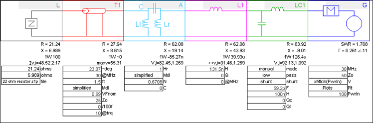
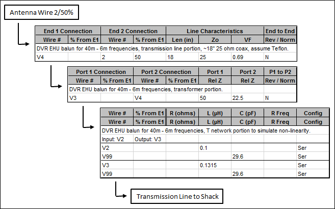
In SimSmith the "load" side is on the left and the "input" side is on the right. So working backwards from the load on the left, first there is an 18 inch (estimated) length of Zo 25 ohm, VF 0.69 transmission line. That is preceded by an ideal transformer with a 0.6708 turns ratio, the equivalent of a 22.5:50 ohm (load:input) impedance ratio. (A 22.5:50 Z ratio is fraction 0.45; Sqrt(0.45)=0.6708. In hindsight I suspect that the load:input turns ratio of the actual balun is 2:3 which equates to a Z ratio of 22.2:50.) Finally there is an
L-C-L "T" network which is used to simulate the various stray capacitance and inductance values in the real balun and associated wiring.So how close is the simulation circuit? This Smith chart shows the modeled (simulated) response as a blue solid trace. It overlays the blue dotted measured response almost perfectly. Both were with the same load, the 22 ohm resistor placed across the brushes.
As for the AutoEZ model, here is a diagram showing the equivalence between the SimSmith circuit elements and the EZNEC insertion objects used to implement the SimSmith circuit.
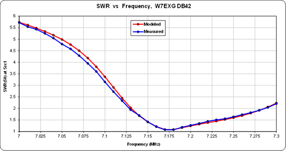
Having a frequency-agile "effective" insulation thickness as described in the previous section, along with a realistic balun model, means that it is possible to obtain very good correlation between measured and modeled SWR on multiple bands. For example, here is a comparison on 40m for a DB42 mounted at 58 feet above desert soil. Measurement data courtesy W7EXG, taken at the shack end of his transmission line using a RigExpert device.
Although not many hams have the ability to verify this, the assumption is that if the model yields impedance/SWR data that has a good correlation to measurements then the pattern data will also be realistic. And if that is so then the modeled patterns can be manipulated with reasonable confidence that the actual antenna will show similar performance.
Modifying the Patterns
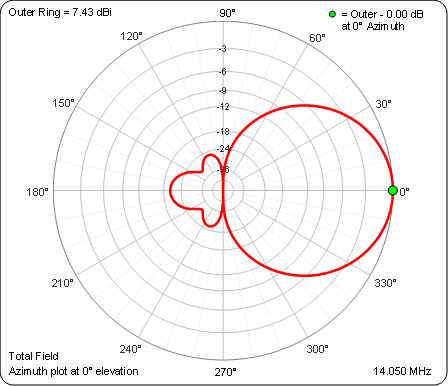
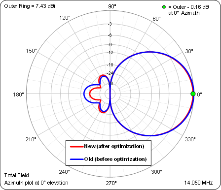
Using the AutoEZ optimizer to tweak the effective insulation thickness is a nice convenience but the real benefit of that tool lies in modifying the azimuth and/or elevation radiation patterns to suit your requirements on a given band.Still working with the DB18E as an example, suppose your interest is primarily CW on the low end of 20m. Here's the Free Space azimuth pattern (elevation 0°) at 14.050 MHz with the shack-to-antenna transmission lines temporarily removed.
Now further suppose that you'd like to improve the F/B (now 20 dB) but not at the expense of making the other rear lobes larger. You'd also like to improve the SWR a bit (now 1.36) and to accomplish both objectives you are willing to give up just a little gain.
On the Variables tab, set the frequency to 14.050 and make sure F18=TRUE. That will display the tape lengths for that frequency under "(modeled)". Type those lengths, at least the integer portions, as the values for K, L, and M. You need not be overly precise, the idea is just to give the optimizer a good starting point as opposed to starting with tape lengths for some other band. Set F18=FALSE.
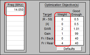
Click the Optimizer Setup button, select K, L, and M, then OK. On the Optimize tab change the frequency to 14.050 and set the target weights to perhaps something like this.
Click Start. If the optimizer stops after just a few trials it's a sure sign that you forgot to change F18 from TRUE to FALSE. If F18=TRUE, when the optimizer runs through the first few trials it won't see any change in the response because, although it is modifying the values for K, L, and M, doing so has no effect. Those variables are ignored if F18=TRUE. So the optimizer gives up. It's almost certain that you will make that mistake at least a few times. Just change F18 on the Variables tab, return to the Optimize tab, and click Start. No need to go through the optimizer setup again, the correct variables have already been selected.
When the optimizer finishes you'll see that the F/R has been improved from 20 dB to 24 dB. (F/R is the range from 90° to 270° azimuth angle whereas F/B is exactly 180° only.) The SWR is also better (now 1.02) and to do both cost you less than 0.2 dBi in forward gain. Here's a comparison of the new and old patterns.
If that is not satisfactory you can modify the optimizer target weights and click Start again. Once you are happy with the new pattern you'll probably want to modify the 20m tape length table row so you can check the patterns on other frequencies while having the lengths be scaled automatically. In other words, you want to scale the lengths from your new settings at 14.050 back to the band segment start at 13.85 so that AutoEZ can automatically scale from there to any other frequency in the 20m band.
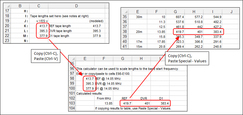
At the bottom of the scratch pad area on the Variables tab, below the Bidirectional tape lengths table, there's a little calculator to do the math for you. To use that calculator follow these steps:
In pictures:
- Select the values for K, L, and M (cells C20-C22) and press Ctrl-C to copy.
- Select cell E98 and press Ctrl-V to Paste. The correct band start values will appear in cells G103-I103.
- Select those cells, G103-I103, and press Ctrl-C to Copy.
- Scroll up, select cell G38, and Paste Special - Values (not normal Paste) into cells G38-I38.
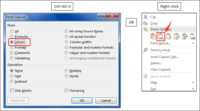
The reason for Paste Special - Values is because there are formulas in cells G103-I103. You don't want to paste the formulas, you want to paste only the calculated results - the values of the copied cells. To do a Paste Special - Values you have two options: a) Select the target cell, press
Ctrl-Alt-V , select "Values" in the dialog window, click OK; or b)Right-click on the target cell and click the Values icon from the context menu.
If you forget and do a regular paste you'll see either "0" or "#VALUE!" in the table row. That's not the end of the world. Just re-copy from the calculator and this time do a Paste Special - Values into the table.
As a last step set F18=TRUE. If you've done everything correctly what you now see under "(modeled)" should be exactly the same as the K, L, M values. Now you can run a frequency sweep over the entire 20m band and the tape lengths will scale correctly at each frequency in the sweep.
This has been a very brief and somewhat contrived example. For more information see the separate Using the Optimizer web page.