Examples of using AutoEZ have been created from time to time to address questions raised on various forums and reflectors. This is a collection of such examples, in some cases slightly edited. Step by step instructions are omitted to maintain brevity.
Using the Optimizer for Yagi Design
Greg Ordy, W8WWV, used the optimizer to design a 10m Yagi on behalf of K8AZ. They very kindly gave me permission to pass along the notes Greg made during the design process.
Preliminary report (PDF, 205 KB)
Final report (PDF, 1.02 MB)
And Jeff Blaine, AC0C, used the optimizer to help design a pair of Yagis for 17m and 12m. He documented his work via one of his web pages.
Coax Lengths for Feeding a Yagi Stack
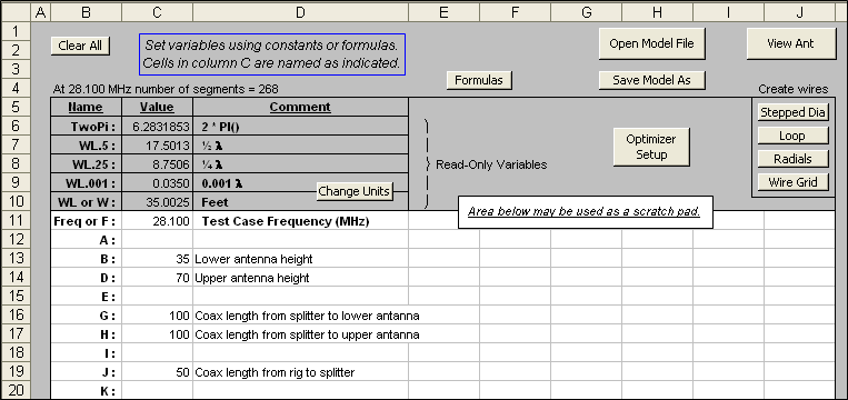
N7TR asked about feedlines for use with a stack of mono-band Yagis and how critical it is to have equal coax lengths, specifically with a StackMaster II and Davis RF Bury-Flex.Using AutoEZ I put together a model with two generic 10m 4-element Yagis stacked at 35 and 70 feet (1 λ and 2 λ on 10m). Each is initially fed with 100 ft of Bury-Flex from the respective feedpoints back to a simulated StackMaster II, modeled as an ideal transformer. From there an additional run of 50 ft of Bury-Flex goes back to the rig.
All of those dimensions are adjustable. Here's a screen grab of the AutoEZ "Variables" sheet.
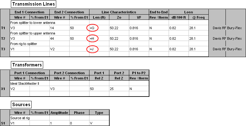
And here are all the "non-antenna" parts of the model. Signal flow is from V1 (source) to V2 (splitter input) to V3 (splitter output) to Yagi feedpoints (Wire 14 / 50% and Wire 44 / 50%).
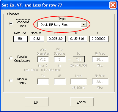
The Zo/VF/Loss values for Bury-Flex were automatically entered using this dialog window. All three characteristics will change if the frequency is changed.
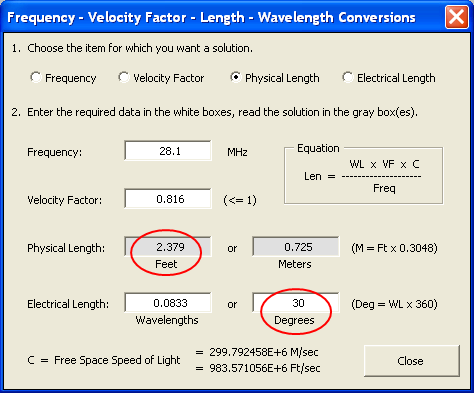
Then I used this dialog to calculate what 30 electrical degrees (an arbitrary choice) would be in feet, using the VF of Bury-Flex at 28.1 MHz.
Finally, I set up a "variable sweep" to change the length of line to the upper antenna by steps equivalent to 30 degrees. That means I'm simulating a mismatch in the line lengths, starting with no mismatch and ending at 180 degrees of mismatch.
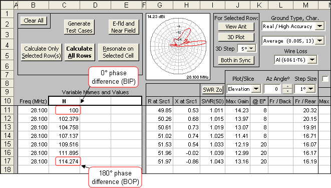
After calculating all the rows this is what the "Patterns" sheet shows. On that sheet you can use the spin button to "watch the movie" of the changing patterns as the mismatch in line lengths grows.
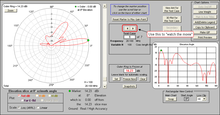
To demonstrate use of the spin button, here's an animated gif. The changing value of variable "H" can be seen in the lower-right corner. The outer ring has been frozen so that the pattern magnitudes as well as shapes may be compared.
Here's the model file used in the above study. (Note that you can't just click on the link to open the model. Save it to your computer then open it from within AutoEZ, as explained in Step 3 of the Quick Start guide.)
Because of the large number of segments you won't be able to use the free demo version of AutoEZ to calculate this model. However, you can modify the model geometry by manually changing one or more variable values, perhaps changing the antenna heights and/or the coax lengths to match your situation. You can then use the View Ant button to view the modified model, which means that AutoEZ will create a temporary .ez format file, pass that file to EZNEC, and invoke the EZNEC viewer. You can then use the EZNEC "FF Plot" button to show the pattern for that particular set of variable values.
As mentioned, the antennas in this model are just generic 10m Yagis that I happened to have on hand.
Coupled Yagis on Separate Towers
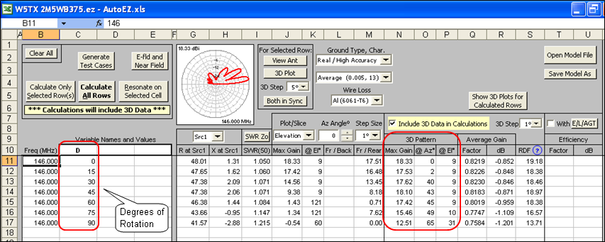
A question was asked about putting two mono-band Yagis at the same height on separate towers. I modeled each at 1.5 λ above real/average ground, fed in phase, separated horizontally by 1.5 λ, with each antenna being rotated by amount "D" degrees.
Here's the EZNEC view, looking straight down from above, as "D" is incremented from 0° to 90° in 15° steps. With most browsers you can use Esc to stop the animation and F5 to restart.
Because the resulting pattern is so convoluted with "D" at anything other than 0° it helps to run a 3D calculation for each test case and then see where the max gain is in terms of Az/El angles. In this AutoEZ screen grab the 3D results are enclosed in red on the right. Notice that at anything other than 0° of rotation the azimuth angle of the max gain point doesn't have much to do with the amount of Yagi rotation.
For most of the test cases the max gain is at 9° elevation, so here is what the azimuth pattern looks like at 9° elevation as "D" is varied from 0° to 90°. The outer ring has been frozen so you can see the difference in gain as well as the difference in pattern shape.
And here is the azimuth pattern at 31° elevation when both antennas are pointing at 90° azimuth. This is the same as the last frame of the above animation except that the elevation angle is 31° instead of 9°.

If the two towers are on a North-South line, with both antennas at 1.5 λ above real/average ground (which puts the TOA at 9° elevation) and the towers are separated by 1.5 λ, here's a comparison of the azimuth patterns at 9° elevation. The blue trace shows both antennas facing East and the red trace shows both antennas facing NE.
The NE facing antennas produce a pattern which is comparable to the broadside pattern. One might even say that the pattern is better. The max gain is down by only an insignificant 0.20 dB and there is only a single large sidelobe.
I then wanted to see what would happen if the spacing between the towers was changed. In this animation the towers are still on a North-South line, both antennas are pointed NE, but the spacing between the towers is varied from 0.75 λ to 4.0 λ. Look in the lower right corner to see the spacing (variable "S") in wavelengths.
Another way to look at things is to plot the max gain vs the tower spacing. In the first frame of the animation above the tower spacing is 0.75 λ (S=0.75). The outer ring is frozen at 18.42 dBi and with S=0.75 the max gain is down 3.56 dB from the outer ring, or 14.86 dBi. In the chart below the first data point is for S=0.75 and the dBi value is 14.86. Other data points show the max gain at different tower spacings.
The S=1.5 λ spacing is a good compromise between max gain and clean pattern.
Modeling an 80m Broadband Dipole
K9YC described a technique for building a broadband 80m dipole. Paraphrasing, "... tune the antenna for 3675 kHz. Feed it with a half wave of 50 ohm line beginning at the antenna, then a quarter wave of 75 ohm cable ..."
For those of you who have AutoEZ here's a step-by-step guide. Start by defining a simple dipole using a variable for the length. Variable "L" was used in this example, any variable name will do.
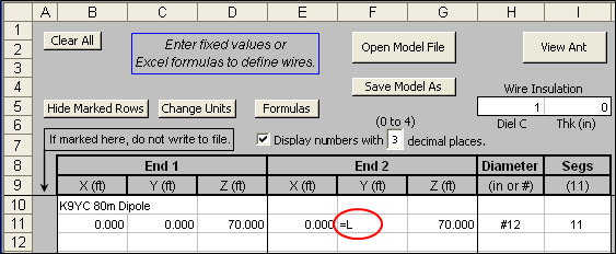
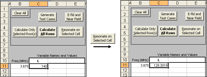
Tab to the Insr Objs sheet and make sure the source is set to Wire 1 / 50%. Tab to the Calculate sheet, set the frequency to 3.675 and give "L" an initial value of something in the neighborhood of a half-wavelength on 80m. With cell C11 still selected click the Resonate on Selected Cell button. The value for "L" will be automatically reset to produce resonance, ~129.3 ft in this example. This was for #12 copper wire at 70 ft over Real/Average ground. Your value will vary depending on the modeling parameters.
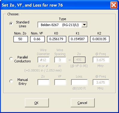
Now add the two transmission line segments that Jim described. In this screen shot T1 is the 180° (half-wave) segment of 50 ohm line, T2 is the 90° (quarter-wave) segment of 75 ohm line. Change the source placement to virtual wire "V1". The connection sequence is V1 (source) to 75-ohm RG-11 to V2 to 50-ohm RG-213 to antenna feedpoint (Wire 1 / 50%).
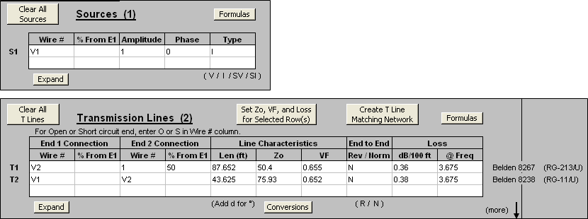
The line characteristics were automatically entered using the Set Zo, VF, and Loss button which shows this dialog. You can choose from roughly 100 different built-in line types.
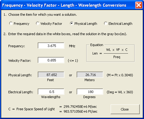
For the precise physical lengths corresponding to 180° and 90° you need not dig out your pocket calculator. You can click the Conversions button which shows this dialog.
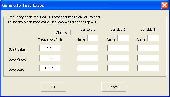
Now tab back to the Calculate sheet and use the Generate Test Cases button to set up a frequency sweep from 3.5 to 4.0 MHz.
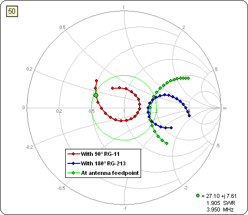
Click Calculate All Rows then tab to the Smith sheet. You'll see this red trace which shows the impedance values at the input (toward the shack) end of the 75 ohm section. I captured the other traces by doing intermediate calculations as the model was being built. The green dot marker on the red trace at 3.950 MHz shows that almost the entire 80m band is within the 2:1 SWR circle.
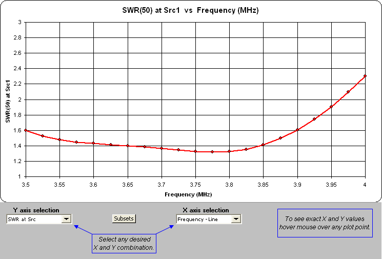
And here's a conventional SWR chart as produced via the Custom sheet tab.
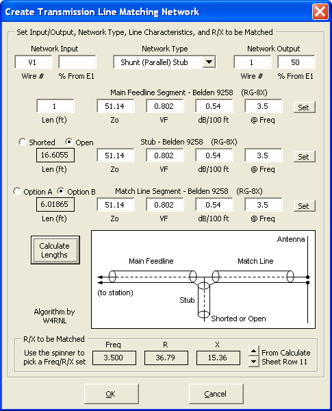
Jim also described how to use the SimSmith tool to design various types of matching networks. AutoEZ has similar capabilities, the difference being that AutoEZ will calculate the correct component values and then add the network to the model. For example, this dialog is used to implement series section or stub transmission line matching networks.
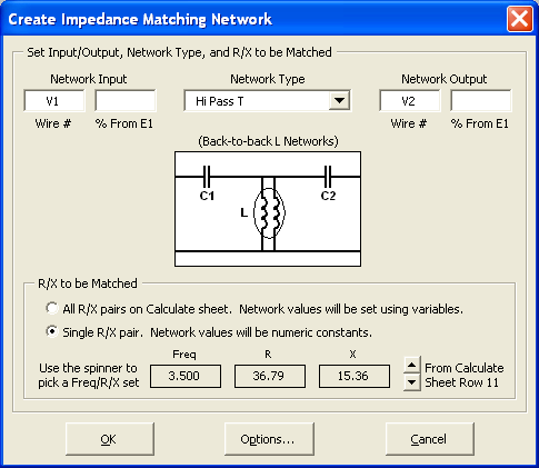
And this one is used to automatically calculate and add T, Pi, and L discrete component networks.
Later in the discussion G3TXQ wrote:
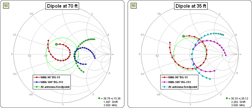
>>> It's worth mentioning that Jim's method needs the dipole to be at a reasonable height - 40ft or more - to avoid having a low resonant feedpoint resistance. Once you go much lower than 40ft, and the resonant impedance falls below about 55 Ohms, the SWR will stay *above* 2:1 all across the band.
Here's a visual of the situation Steve describes.
If you'd like to play with this model without bothering to build it from scratch here's the AutoEZ format (.weq) model file.
Vertical Dipole, Pattern vs Base Height
Concerning measurements made by K9YC on a vertical dipole, VK3QI wrote:
>>> Are you really measuring what DXers are really after when comparing vertical antennas at different heights above ground and ground mounted?
Putting aside for the moment the distinction between measuring and modeling, I wanted to investigate what VK3QI said about "DX angles" (in this case 10°) vs "zero" angle. First thing I did was create an adjustable vertical dipole model that also has ground conditions that can be set via a variable. Here's the AutoEZ "Variables" sheet showing (to start) the base (variable B) at 20 ft, the length (variable D) at 35 ft, and the ground type (variable G) as "Average".
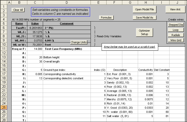
With those starting conditions I used the Resonate on Selected Cell button to reset the length (variable D). After that the length was not changed.

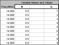
Then I set up a series of test cases with the base at 0.5 ft and with the ground characteristics varying through all the non-water choices, from Extremely Poor to Very Good, per the EZNEC definitions of such.
Here's an animated gif showing the results. The value for "G" (Ground type index) may be seen in the lower right corner.
As the ground gets better the gain at 10° gets better (pretty much). Then I ran a similar series of test cases with the base of the dipole at 40 ft. Again, look in the lower right corner to see the "G" value for any given frame of the animation.
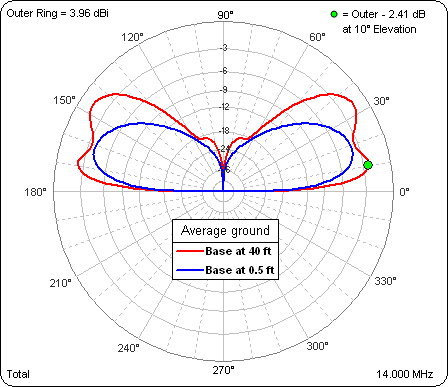
That was interesting. With the base at 40 ft the gain at 10° gets worse as the ground gets better. More of the energy is going into the second (higher) lobe. However, note that the outer ring is the same for both these animations so you can compare magnitudes as well as pattern shapes. For any given ground type the "DX angle" (10°) gain is always higher for the higher dipole. For example, here's a comparison for Average ground.
So that seems to address the first point that VK3QI made. Gain at "DX angles" (in this case 10°) gets better as the dipole is raised and it doesn't matter what the ground conditions are. Now for his point about actual measurements.
VK3QI also wrote:
>>> Measuring a vertical at another location 5 miles away, but at the same relative height is really measuring the ability of the vertical antenna to couple to the ground to produce a vertically polarised ground wave.
And that seems to be in regards to page 76 from the K9YC presentation Vertical Antenna Mounting Height:
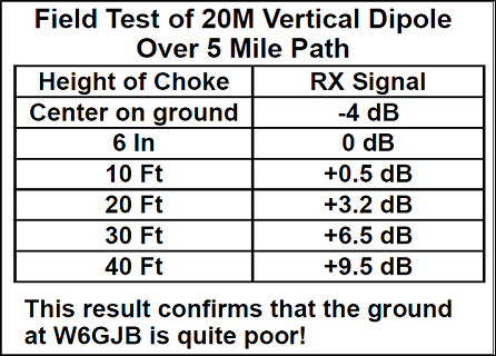
K9YC measured an increase in gain of 9.5 dB as the dipole base was raised from 0.5 ft to 40 ft. If both he and the 3 watt transmitter at W6GJB had been located on the wheat fields of Kansas that would have been one thing, but they are both in the Santa Cruz mountains and I'm betting it's not exactly 5 miles of flat ground (as NEC assumes) between them. Hence I'm not sure how to use NEC to verify the K9YC measurements since there is no Far Field at an elevation of 0°. So I fudged a bit.
Here's an animation with the green dot marker at 1° elevation, not exactly the same as equal heights but close. The ground type is fixed at Very Poor per K9YC's comments. The dipole base height (variable "B", lower right corner) ranges through 0.5, 10, 20, 30, and 40 ft.
As the base height is raised the gain at 1° increases by about 6.6 dB (from -19.34 dBi to -12.72 dBi). That's not identical to the measured increase of 9.5 dB but it seems to verify that the gain at "ground level" (almost) should increase as the dipole height is increased, which seems to corroborate what K9YC measured.
Here's the model file I used if anyone else would like to play with it. (Note that you can't just click on the link to open the model. Save it to your computer then open it from within AutoEZ, as explained in Step 3 of the AutoEZ Quick Start guide.)
This model will work just fine with the free demo version of AutoEZ.